The purpose of this document is to summarize the ideas from the titular paper and gain experience with the fundamentals of pharmacokinetics in the R programming language. Also, some of the examples which were lacking in detail have been fleshed out for a clearer presentation.

Basic Definitions + History

Pharmacokinetics (PK)
Studying the relationships between the physiological characteristics of an individual and observed drug exposure or response.

• This should be done in a way that accounts for between-subject-variability (BSV) by considering population-level parameter value distributions.
  • Initially two approaches were taken (i) combining all the data from individuals (the “naive pooled approach”), or (ii) by fitting all individuals separately and taking parameter means (the “two-stage approach”). Both approaches becoming increasingly problematic as the data collection becomes sparser and sloppier (i.e., real-world data).
  • A more accurate approach was taken by Sheiner et al. 1972 by accounting for BSV through the covariance of model parameters. This can yield informed estimates of the variability of drug exposure with age and weight as well as within the general populations.
  • Such information is critical to “inform the initial selection of doses to test, modify or personalize dosage for subpopulations of patients, and evaluate the the appropriateness of study designs.”

Pharmacodynamics (PD)
Studying the relationship between drug concentration, including its intrinsic dynamics, and the observed physiological response.

Model
A simplified representations of a system designed to provide knowledge or understanding of the system.

• “All models are wrong, some are useful”.

  • A credible and high-fidelity choice of specific model for a specific purpose requires that it justified and defendable.

    • “Credible models are ones for which the assumptions made in the construction are understood and clearly stated”

    • “Fidelity is gauged by comparing the model to components of the system (reality) that are considered important (note that fidelity does not always imply credibility)”

  • Model development should involve ranking credible models according to their fidelity.

Summary:

PK Models - How long does a drug stay in the body? How does that vary within a population?

PD Models - What does a drug do while it is in the body?

PK models should

• “provide a basis for describing and understanding the time-course of drug exposure and response after the administration of different doses or formulations of a drug to individuals”

• “provide a means for estimating the associated parameters such as clearance and volume of distribution of a drug”

  • “Population models should yield parameter estimates which can be compared to previous assessments to determine consistency between studies or patient populations.”

The data that is used in model parametertizaton can also be compared with those relating to other drugs in the same therapeutic class, as a means of evaluating the development potential of a new therapeutic agent.

PK models

• Usually built from interconnected “compartments” where the concentration is assumed to be uniform and the drug may move from one compartment to the other.

  • Physiology-based PK models (PBPK) have compartments that map onto anatomically defined parts of the body (e.g., organs, blood, connective tissue).

  • PBPK models often have more compartments, which makes parameter estimation more difficult in clinical setting. However they can yield more insight into how physiological perturbations and disease might influence drug distribution, this can be useful in translating findings from preclinical to clinical settings

PKPD Models

These model additionally include a model of the effects of the drug, which is critical in predicting clinical outcomes. Developing a PD model requires knowledge of the concentration-effect relationship and choice of a typical effect size for a “successful” treatment. Then, using the population-level PK model, we can determine a probability of success within a cohort.

• “Exposure–response models are a class of PKPD models wherein the independent variable is not time, but rather, a metric describing drug exposure at steady-state (e.g., dose, area under the curve ($\text{A.U.C}$), or peak plasma concentration ($C_{\text{max}}$)).”

Disease progression models

Describe the time course of a diseases evolution and account for BSV in disease progression, crucially these must be developed from a placebo group. They can then be linked to PD/PKPD to determine the efficacy of drug treatment.

Meta-models

Meaning “the analysis of analyses”, these are analyses of aggregated results from many individual studies that are critical for decision making purposes. Their implementation is non-trivial due a variety of considerations related to study and model design.

Bayesian Averaging

Bayesian approaches are very useful for model selection when multiple models exist and there is uncertainty about which might be best suited.

Some Examples of Population Models

Preliminaries

The three main components of population models are:

1. Structural Models - functions that describe the time course of a measured response, which can be represented implicitly as algebraic or differential equations.

2. Stochastic Models - descriptions of the variability or random effects in the observed data

3. Covariate Models - descriptions of the influence of factors such as demographics or disease on the individual time course of the response

A model can only be as good as the data it was fit to. Data coming from clinical trials can be very heterogeneous in quality, sampling frequency, and units. These all introduce non-negligible challenges for fitting PK model in a high quality manner.

Models

Structural Models

The simplest PK model is arguably a one-compartment model where a single dose of drug is administered intravenously to a compartment with volume $V$. The time-dependent concentration of drug, $C(t)$, can be expressed as either a differential equation or algebraic equation. That is

where $k>0$ is the clearance rate of the drug from the “body” compartment. In the differential equation, time is unambiguously the independent variable. However, once it is solved and we have the algebraic expression it is also possible to vary any of the model parameters at some fixed time and ask how some model outcome varies.

Because this is a linear ODE, if multiple doses are administered at a set of times ${t_j}$ then we may exploit the superposition of solutions to obtain

or, more generally, for a generic time-dependent dose delivery regimen, $\text{dose}(t)$, we may use the convolution theorem to obtain

where discrete injections could be modeled as Dirac delta functions.

Stochastic Models

Population models can account for a drug’s BSV and between-occasion variability. We can write down a simple formalism to describe this variability as a random parameter $p$ consisting of the sum of a population mean $\theta$ and a random effect $\eta$, i.e.,

where $\eta$ is assumed to have zero mean and variance $\omega$ (and is often assumed to be normally or log-normally distributed).

Accounting for such variability is is critical for determining the suitability of a drug for therapeutic purposes. For example, a drug with narrow therapeutic window but large variability would not be a good candidate for bringing to market as it is likely that few people would benefit from it.

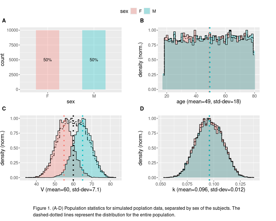
To get more concrete idea of what this might mean, we can generate an artificial population by modeling individuals as a one-compartment models. Lets assume that we can find a population of subjects that are uniformly distributed in age, with volume that is normally distributed (but the two different sexes are sampled from distributions with different means), and a clearance rate that is roughly normally distributed (independent of sex). Data for such a population is generated and its statistics are plotted in the code chunk below.

#library(ggstats)
library(ggplot2)
#library(dplyr)
library(ggpubr)
library(latex2exp)

source('util.R')

n<-2e4 #number of subjects

pop <- data.frame(
     #roughly half females and males
     sex=factor(c(rep("F", each=floor(n/2)),rep("M", each=ceiling(n/2)) )),
     #uniformly distributed ages 18-80 years old
     age=runif(n,18,80),
     #assume males have 10 more volume units than females
     V=c(
       rnorm(floor(n/2), mean=55, sd=5),
       rnorm(ceiling(n/2), mean=65, sd=5)
       )
 )

#clearance rate is normally-distributed with a mean that decreases with age - a covariate effect
pop$k=rnorm(n, 11.2-3.2*(pop$age-18)/62, 0.8)/1e2


captioned(plot_population_stats(pop,  group=sex, total_pop=T, group_means=T), 
          text="Figure 1. (A-D) Population statistics for simulated poplation data, separated by sex of the subjects. The dashed-dotted lines represent the distribution for the entire population." )

Now, suppose a certain drug needs to be above a threshold concentration, $C_{\text{thresh}}$, to have an effect, but if its concentration remains too elevated for too long then it can start to cause negative side effects. Using the one-compartment model we can compute the time it takes for the concentration to fall below $C_{\text{thresh}}$, this is given by the expression

where the max operation is use to account for scenarios where the initial concentration is already below $C_{\text{thresh}}$. Then we can quantify the extent to which concentration is elevated using the area under the curve, $\text{A.U.C.}$, which accounts for both the amount of time a drug has non-negligible concentration as well as how high the concentration is. For the one-compartment model, this can be computed as

where we note that $\lim_{t\to\infty}A.U.C(t)=\frac{\text{dose}}{V} \frac{1}{k}$. As a simple example, we assume that in order to generate therapeutic benefit we need $A.U.C(t_{thresh})$ greater than some threshold while also having $A.U.C(\infty)$ less than another threshold, which we denote as the therapeutic window of the drug in this scenario.

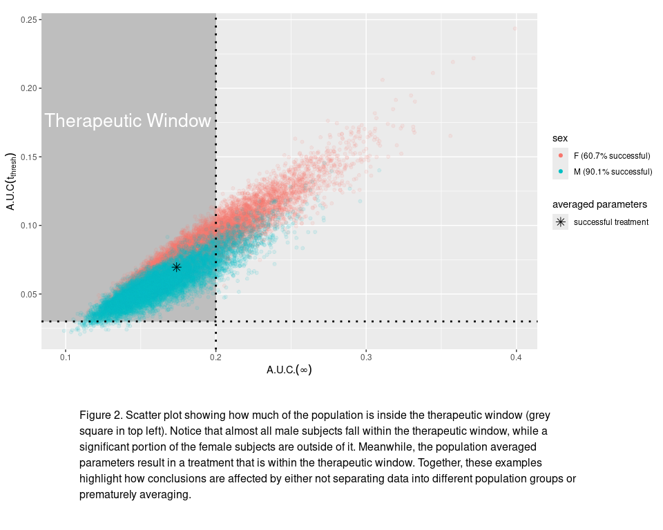
In the code chunk below, we compute these $A.U.C.$ values for our simulated population and then assess what proportion of the population receives a therapeutically “successful” treatment (i.e., with $A.U.C(t_{thresh})$ large enough for therapeutic benefit but with $A.U.C.(\infty)$ not too large to cause significant side effects). As we can see from the figure, by simply using the population averaged PK parameters we predict a successful treatment whereas accounting for the variability in volume and clearance rate we can see a more nuanced picture where treatment is successful for approximately 60% (90%) of females (males) in the population. These population-dependent predictions are completely missed if the stochastic nature of BSV is not accounted for.

source('one_compartment.R')
C_thresh<-0.01

side_effects_thresh <- 0.2
therapeutic_thresh <- 0.03


#compute AUC for t=infinity and t=t_thresh
pop_dosage<-compute_AUCs(pop, C_thresh)




plot<-ggplot(pop_dosage, aes(x=auc_infinity, y=auc_thresh, color=sex))+
  annotate("rect", xmin=-Inf, xmax=side_effects_thresh, ymin=therapeutic_thresh, ymax=Inf, fill="grey")+
  annotate("text", x = 0.42*(side_effects_thresh-min(pop_dosage$auc_infinity))+min(pop_dosage$auc_infinity) ,
           y = 0.7*(max(pop_dosage$auc_thresh)-min(pop_dosage$auc_thresh))+min(pop_dosage$auc_thresh),
           label = "Therapeutic Window", color="white", size=7)+
  geom_point(alpha=min(2e3/n,1))+
  filtered_stats_in_legend(pop_dosage, cond=auc_infinity<side_effects_thresh & auc_thresh>therapeutic_thresh, group=sex,
                           scale=scale_color_discrete)+
  guides(color = guide_legend(override.aes = list(alpha = 1) ) )+
 geom_cross_line(x=side_effects_thresh, y=therapeutic_thresh, linetype="dotted",
                 linewidth=1, show.legend = F,  color="black")+
 average_geom_point(pop, post_process=function(df) compute_AUCs(df,C_thresh),
                fill=function(average)
                  ifelse(with(average, auc_infinity<side_effects_thresh & auc_thresh>therapeutic_thresh),
                  "successful treatment", "failed treatment")
                , color="black", size=3, shape=8)+
  labs(x=TeX("$A.U.C.(\\infty)$"), y=TeX("$A.U.C(t_{thresh})$"))


#generate scatter plot
captioned(plot,
text="Figure 2. Scatter plot showing how much of the population is inside the therapeutic window (grey square in top left). Notice that almost all male subjects fall within the therapeutic window, while a significant portion of the female subjects are outside of it. Meanwhile, the population averaged parameters result in a treatment that is within the therapeutic window. Together, these examples highlight how conclusions are affected by either not separating data into different population groups or prematurely averaging.", height=c(3,1))

Covariate Models

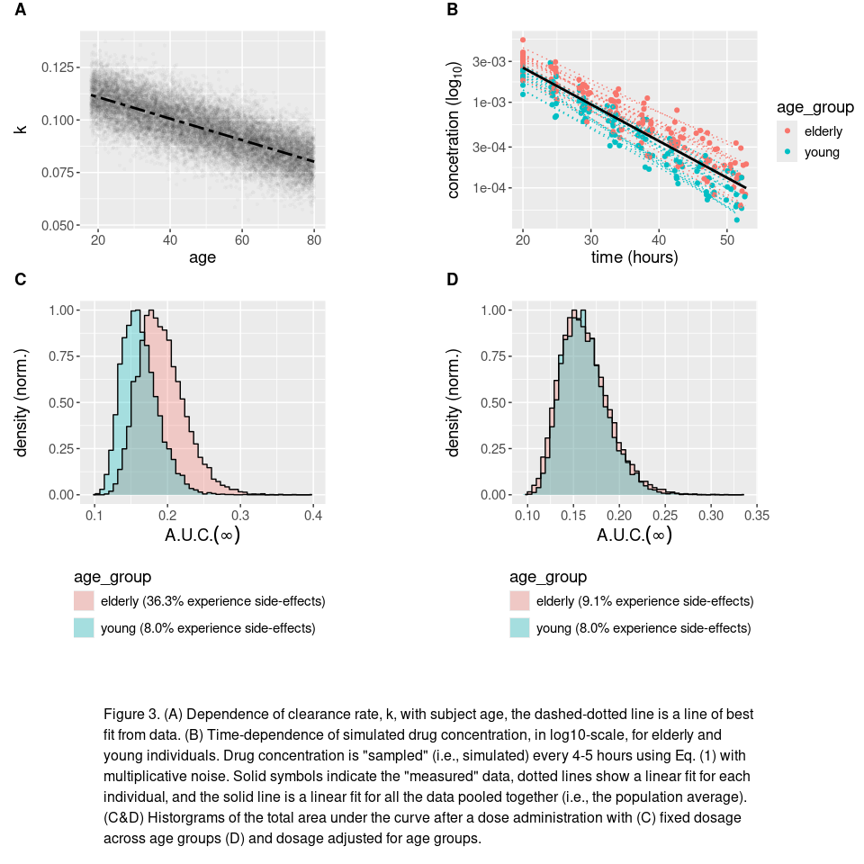
If you looked carefully in the first code chunk you may have noticed that we made clearance rate depend linearly on the age of an individual. This is an example of a covariate population model, where the random value of different parameters are correlated. In this specific instance, we have chosen

where $m$ and $b$ are constants and $\eta$ is normally distributed random effect with a variance of $6.4\times10^{-5}$ (see the Fig. 3A for illustration).

More generally, a correlation between the $\text{i}^\text{th}$ and $\text{j}^\text{th}$ random parameters can be expressed by a formalism given by

where $\theta_i$ & $\theta_j$ are the population means as before, $g_i$ & $g_j$ are multi-dimensional functions, and the values $X_k$ are covariate random variables (i.e., random variables that allow the parameter values to have some degree of dependence on one another). For the previous example, this formalism reduces to

We note that this example uses linear functions for $g_{\text{age}}$ and $g_k$, but in general this need not be the case.

Covariance between parameters can have profound implications for therapeutic outcomes of a drug within sub-populations (e.g., people with certain conditions, within different age ranges, or living specific lifestyles). In our previous example clearance decreases with age, which accordingly results longer-lasting concentration levels of drug concentration to the one-compartment model makes consider how

source('one_compartment.R')
source('util.R')

p1<-ggplot(pop, aes(x=age, y=k))+
  geom_point(stroke=0, alpha=min(5e2/n,.2))+
  geom_smooth(formula = y~x, method='lm', color="black",linetype=6)

age_thresh<-45
pop_dosage$age_group=factor(sapply(pop_dosage$age, function(age) if(age>age_thresh){"elderly"}else{"young"}))





sub_pop_timeseries<-bind_with(sub_sample(pop_dosage, 30), 
                              mutate(concentration_sample(k, V, t_sample=cumsum(c(20,runif(7, 4,5)))),
                                     age_group=age_group),
                               .id="id")


p2<-ggplot(sub_pop_timeseries,aes(x=time,y=concentration, color=age_group), log10="y")+
  geom_point()+ scale_y_continuous(trans='log10')+
  geom_smooth_group_and_mean(group=id, formula = y ~ x, method="lm", se=F, show.legend = F)+
  labs(y=TeX("concetration ($\\log_{10}$)"), x="time (hours)")



AUC_by_age_group<-summarise(group_by(pop_dosage,age_group), mean=mean(auc_infinity))
adjusted_dose<-with(AUC_by_age_group, min(mean)/max(mean))

pop_adjusted_dosage<-data.frame(pop_dosage)

inds<-which(pop_dosage$age_group=="elderly")

pop_adjusted_dosage[inds,]<-compute_AUCs(pop_dosage[inds,], C_thresh, dose=adjusted_dose)



p34<-lapply( list(pop_dosage, pop_adjusted_dosage), 
             function(data){

                plot_population_stats(data, column=auc_infinity, group=age_group,
                                      group_means = F, stats_in_label=F,
                                      x_label=TeX("$A.U.C.(\\infty)$"), margin=unit(c(1,0,0,0), 'cm'))+
                   filtered_stats_in_legend(data, cond=auc_infinity>=side_effects_thresh, group=age_group,
                                          success_string="%s (%0.1f%% experience side-effects)")+
                   guides(fill=guide_legend(ncol=1, title.position="top", position="bottom"))

          })

captioned(
          
          ggarrange(plotlist=lapply(c(list(p1,p2),p34),
                                    function(p) p+theme(plot.margin=unit(c(0.4,0,0.6,0.4), 'cm'),
                                                        text = element_text(size = 14) )
                                    ),
                    nrow=2, ncol=2, align='v', labels="AUTO", vjust=-0.13, hjust=-1.25, heights=c(1,1.4)),
          
          text="Figure 3. (A) Dependence of clearance rate, k, with subject age, the dashed-dotted line is a line of best fit from data. (B) Time-dependence of simulated drug concentration, in log10-scale, for elderly and young individuals. Drug concentration is \"sampled\" (i.e., simulated) every 4-5 hours using Eq. (1) with multiplicative noise. Solid symbols indicate the \"measured\" data, dotted lines show a linear fit for each individual, and the solid line is a linear fit for all the data pooled together (i.e., the population average). (C&D) Historgrams of the total area under the curve after a dose administration with (C) fixed dosage across age groups (D) and dosage adjusted for age groups.",
          heights=c(4,1)
          )